
The canonical example of matrix decompositions, the Principal Components Analysis (PCA), is ubiquitous, with applications in many scientific fields including neuroscience, genomics, climatology, and economics. Increasingly, the data sets available to scientists are in range of hundreds of gigabytes or terabytes, and their analyses are bottle-necked by the computation of the PCA or related low-rank matrix decompositions like the Non-Negative Matrix factorization (NMF). The sheer size of these data sets necessitates distributed analyses. Spark is a natural candidate for implementation of these analyses. Together with my collaborators at Berkeley: Aditya Devarakonda, Michael Mahoney, James Demmel, and with teams at Cray, Inc. and NERSC’s Data Analytic Services group, I have been investigating the performance of Spark at computing scientific matrix decompositions.
We used MLlib and ml-matrix to implement three scientifically useful decompositions: PCA, NMF, and a randomized CX decomposition for column subset selection. After implementing the same algorithms in MPI using standard linear algebra libraries, we characterized the runtime gaps between Spark and MPI. We found that Spark implementations range from 2x to 26x slower than the MPI implementations of the same algorithm. This highlights that there are still opportunities to improve the current support for large-scale linear algebra in Spark.
While there are well-engineered, high-quality HPC codes for computing the classical matrix decompositions in a distributed fashion, these codes are often difficult to deploy without specialized knowledge and skills. In some subfields of scientific computation, like numerical partial differential equations, these knowledge and skills are de rigueur, but in others, the majority of scientists lack sufficient expertise to apply these tools to their problems. As an example, we point out that despite the availability of the CFSR data set— a collection of samples of three-dimensional climate variables collected at 3 to 6 hours intervals over the course of 30+ years— climatologists have largely limited their analyses to 2D slices because of the difficulties involved with loading the entire dataset. The PCA decompositions we computed in the course of our investigations here are the first time that three-dimensional principal components have been extracted from a terabyte-scale subset of this dataset.
What do we mean by “scientific” matrix decompositions? There is a large body of work on using Spark and similar frameworks to compute low-precision stochastic matrix decompositions that are appropriate for machine learning and general statistical analyses. The communication patterns and precision requirements of these decompositions can differ from those of classical matrix decompositions that are used in scientific analyses, like the PCA, which is typically desired to be computed to high precision. We note that randomized algorithms like CX and CUR are also of scientific value, as they can be used to extract interpretable low-rank decompositions with provable approximation guarantees.
There are multiple advantages to implementing these decompositions in Spark. The first, and most attractive, is the accessibility of Spark to scientists who do not have prior experience with distributed computing. But also importantly, unlike traditional MPI-based codes which assume that the data is already present on the computational nodes, and require manual checkpointing, Spark provides an end-to-end system with sophisticated IO support and automatic fault-tolerance. However, because of Spark’s bulk synchronous parallel programming model, we know that the performance of Spark-based matrix decomposition codes will lag behind that of MPI-based codes, even when implementing the same algorithm.
To better understand the trade-offs inherent in using Spark to compute scientific matrix decompositions, we focused on three matrix decompositions motivated by three particular scientific use-cases: PCA, for the analysis of the aforementioned climatic data sets; CX (a randomized column subset selection method), for an interpretable analysis of a mass spectrometry imaging (MSI) data set; and NMF, for the analysis of a collection of sensor readings from the Daya Bay high energy physics experiment. The datasets are described in Table 1.
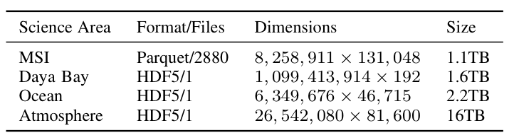
Table 1: Descriptions of the data sets used in our experiments.
For each decomposition, we implemented the same algorithms for PCA, NMF, and CX in C+MPI and in Spark. Our data sets are all “tall-and-skinny” highly rectangular matrices. We used H5Spark, a Spark interface to the HDF5 library developed at NERSC, to load the HDF5 files. The end-to-end (including IO) compute times for the Spark codes and the MPI codes are summarized in Table 2 for different levels of concurrency.
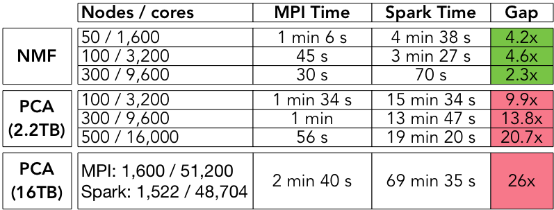
Table 2: summary of Spark and MPI run-times.
The MPI codes range from 2 to 26 times faster than the Spark codes for PCA and NMF. The performance gap is lowest for the NMF algorithm at the highest level of concurrency, and highest for the PCA algorithm at the highest level of concurrency. Briefly, this difference is due to the fact that our NMF algorithm makes one pass over the dataset, so IO is the dominant cost, and this cost decreases as concurrency increases. On the other hand, the PCA algorithm is an iterative algorithm (Lanczos), which makes multiple passes over the dataset, so the dominant cost is due to synchronization and scheduling; these costs increase with the level of concurrency.
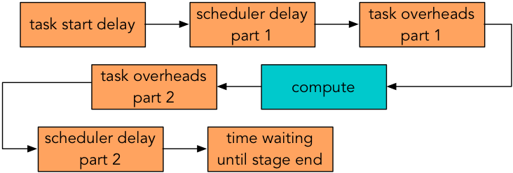
Figure 1: Spark overheads.
Figure 1 summarizes some sources of Spark overhead during each task. Here, “task start delay” measures the time from the start of the stage to the time the task reaches the executor; “scheduler delay” is the time between a task being received and being deserialized plus the time between result serialization and the driver receiving the task’s completion message; “task overhead time” measures the time spent waiting on fetches, executor deserialization, shuffle writing, and serializing results; and “time waiting until stage end” is the time spent waiting for all other tasks in the stage to end.
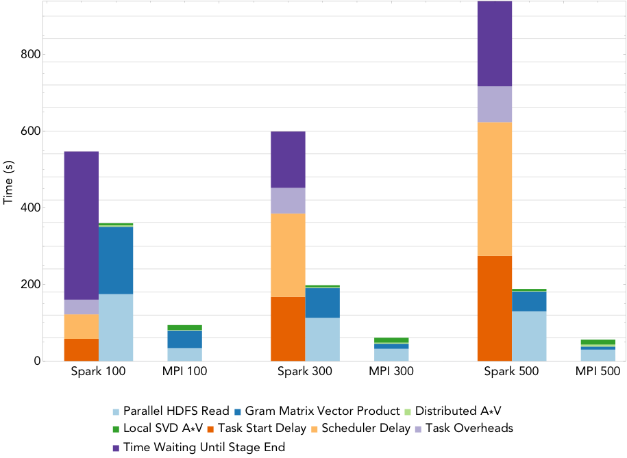
Figure 2: Run times for rank 20 PCA decomposition of the 2.2TB ocean temperature data set on varying number of nodes.
To compute the PCA, we use an iterative algorithm that computes a series of distributed matrix-vector products until convergence to the decomposition is achieved. As the rank of the desired decomposition rises, the number of required matrix-vector products increases. Figure 2 shows the run times for the MPI and Spark codes when computing a rank 20 PCA of the 2.2TB ocean temperature data set on NERSC’s Cori supercomputer, as the level of parallelism increases from 100 nodes (3,200 cores) to 500 nodes (16,000 cores). The overheads are reported as the sum over all stages of the mean overheads for the tasks in each stage. The remaining buckets are computational stages common to both the Spark and MPI implementations. We can see that that the dominant costs of computing the PCA here is the cost of synchronizing and scheduling the distributed matrix-vector products, and these costs increase with the level of concurrency. Comparing just the compute phases, Spark is less than 4 times slower than MPI at all levels of concurrency, with this gap decreasing as concurrency increases.
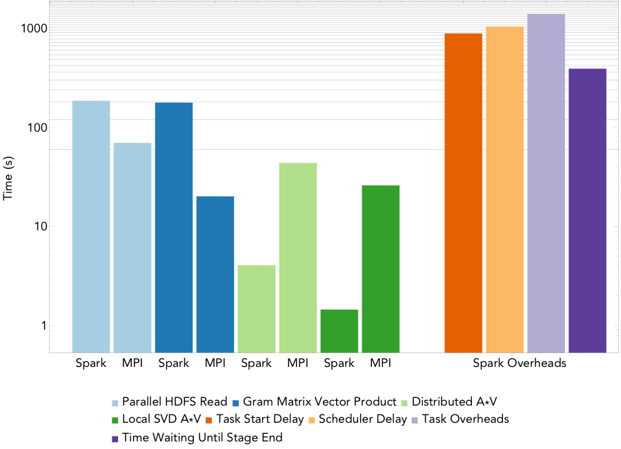
Figure 3: Run times for computing a rank 20 decomposition of the 16TB atmospheric humidity data set on 1522/1600 nodes.
Figure 3 shows the run times for the MPI and Spark codes for PCA at a finer level of granularity for the largest PCA run, computing a rank 20 decomposition of a 16TB atmospheric humidity matrix on 1600 of the 1630 nodes of the Cori supercomputer at NERSC. MPI scaled successfully to all 51200 cores, and Spark managed to launch 1522 of the requested executors, so scaled to 48704 cores. The running time for the Spark implementation is 1.2 hours while that for the MPI implementation is 2.7 minutes. Thus, for this PCA algorithm, Spark’s performance is not comparable to MPI— we note that the algorithm we implemented is the same as the most scalable PCA algorithm currently available in MLlib.
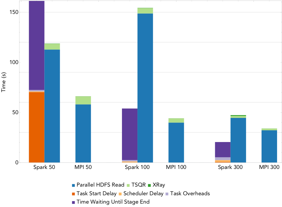
Figure 4: Run times for NMF decomposition of the 1.6TB Daya Bay data set on a varying number of nodes.
By way of comparison, the Spark NMF implementation scales much better. Figure 4 gives the run time breakdowns for NMF run on 50 nodes, 100 nodes, and 300 nodes of Cori (1,600, 3,2000, and 16,000 cores respectively). This implementation uses a slightly modified version of the tall-skinny QR algorithm (TSQR) available in ml-matrix to reduce the dimensionality of the input matrix, and computes the NMF on this much smaller matrix locally on the driver. The TSQR is computed in one pass over the matrix, so the synchronization and scheduling overheads are minimized, and the dominant cost is the IO. The large task start delay in the 50 node case is due to the fact that the cluster is not large enough to hold the entire matrix in memory.
The performance of the CX decomposition falls somewhere in between that of the PCA and the NMF, because the algorithm involves only a few passes (5) over the matrix. Our investigation into the breakdown of the Spark overheads (and how they might be mitigated with more carefully designed algorithms) is on-going. We are also collaborating with climate scientists at LBL in the analysis of the three-dimensional climate trends extracted from the CFSR data.