This gallery contains 6 photos.
A critical part of enabling cities to implement their Vision Zero policies – the goal of the current National Transportation … Continue reading

This gallery contains 6 photos.
A critical part of enabling cities to implement their Vision Zero policies – the goal of the current National Transportation … Continue reading

The West Big Data Innovation Hub (WBDIH) is excited to host a Data Hackathons: Lessons Learned and Best Practices Workshop on September 15 as part of the historic first International Data Week in Denver.
One of four hubs recently launched with funding from the National Science Foundation and leadership from UC Berkeley, University of Washington, and the San Diego Supercomputer Center, the WBDIH builds and strengthens partnerships across industry, academia, nonprofits, and government to address societal challenges.
As mentioned at the WBDIH All Hands Meeting held at UC Berkeley this spring, the workshop will convene hackathon organizers, sponsors, and other stakeholders to share insights about the design, implementation, scalability, and impact of data-focused hackathons. Data hackathon case studies mentioned will cover the WBDIH thematic areas including Metro Data Science, Natural Resources and Hazards, and Precision Medicine, as well as cross-cutting topics.
Funding for Early Career Data Scientists
The September workshop is the second WBDIH hands-on event offering grants for early career data scientists through a collaboration with the Computing Community Consortium (CCC). In June 2016, over 700 data enthusiasts from 25 states and 15 countries gathered in Los Angeles and via livestream for a workshop on The Science of Data-Driven Storytelling. To encourage early career researchers to participate and contribute to the #datascistories and #datahackworkshop communities, the WBDIH has partnered with the CCC to provide funding. Grant Applications for the Data Hackathons Workshop are due Sept. 6, 2016: http://bit.ly/WBDIHtravel.
Remote Participation and Community-Driven Resources
Remote participants are encouraged to join the conversation are share resources at WBDIH.slack.com and #datahackworkshop. More information, including the livestream from 2–5pm MST Sept. 15, will be posted at http://westbigdatahub.org/datahackworkshop and through the WBDIH mailing list.
Share the announcement on Twitter | Retweet the U.S. Chief Data Scientist’s Tweet | Share via Facebook

Each month the Communications of the ACM publishes an invited “Review Article” paper chosen from across the field of Computer Science. These papers are intended to describe new developments of broad significance to the computing field, offer a high-level perspective on a technical area, and highlight unresolved questions and future directions. The June 2016 issue of CACM contains a paper by AMPLab researcher Michael Mahoney and his colleague Petros Driness (of RPI, soon to be Purdue). The paper, “RandNLA: Randomized Numerical Linear Algebra,” describes how randomization offers new benefits for large-scale linear algebra computations such as those that underlie a lot of the machine learning that is developed in the AMPLab and elsewhere.
Randomized Numerical Linear Algebra (RandNLA), a.k.a., Randomized Linear Algebra (RLA), is an interdisciplinary research area that exploits randomization as a computational resource to develop improved algorithms for large-scale linear algebra problems. From a foundational perspective, RandNLA has its roots in theoretical computer science, with deep connections to mathematics (convex analysis, probability theory, metric embedding theory), applied mathematics (scientific computing, signal processing, numerical linear algebra), and theoretical statistics. From an applied “big data” or “data science” perspective, RandNLA is a vital new tool for machine learning, statistics, and data analysis. In addition, well-engineered implementations of RandNLA algorithms, e.g., Blendenpik, have already outperformed highly-optimized software libraries for ubiquitous problems such as least-squares.
Other RandNLA algorithms have good scalability in parallel and distributed environments. In particular, AMPLab postdoc Alex Gittens has led an effort, in collaboration with researchers at Lawrence Berkeley National Laboratory and Cray, Inc., to explore the trade-offs of performing linear algebra computations such as RandNLA low-rank CX/CUR/PCA/NMF approximations at scale using Apache Spark, compared to traditional C and MPI implementations on HPC platforms, on LBNL’s supercomputers versus distributed data center computations. As Alex describes in more detail in his recent AMPLab blog post, this project outlines Spark’s performance on some of the largest scientific data analysis workloads ever attempted with Spark, including using more than 48,000 cores on a supercomputing platform to compute the principal components of a 16TB atmospheric humidity data set.
Here are the key highlights from the CACM article on RandNLA.
1. Randomization isn’t just used to model noise in data; it can be a powerful computational resource to develop algorithms with improved running times and stability properties as well as algorithms that are more interpretable in downstream data science applications.
2. To achieve best results, random sampling of elements or columns/rows must be done carefully; but random projections can be used to transform or rotate the input data to a random basis where simple uniform random sampling of elements or rows/ columns can be successfully applied.
3. Random sketches can be used directly to get low-precision solutions to data science applications; or they can be used indirectly to construct preconditioners for traditional iterative numerical algorithms to get high-precision solutions in scientific computing applications.
More details on RandNLA can be found by clicking here for the full article and the associated video interview.

The canonical example of matrix decompositions, the Principal Components Analysis (PCA), is ubiquitous, with applications in many scientific fields including neuroscience, genomics, climatology, and economics. Increasingly, the data sets available to scientists are in range of hundreds of gigabytes or terabytes, and their analyses are bottle-necked by the computation of the PCA or related low-rank matrix decompositions like the Non-Negative Matrix factorization (NMF). The sheer size of these data sets necessitates distributed analyses. Spark is a natural candidate for implementation of these analyses. Together with my collaborators at Berkeley: Aditya Devarakonda, Michael Mahoney, James Demmel, and with teams at Cray, Inc. and NERSC’s Data Analytic Services group, I have been investigating the performance of Spark at computing scientific matrix decompositions.
We used MLlib and ml-matrix to implement three scientifically useful decompositions: PCA, NMF, and a randomized CX decomposition for column subset selection. After implementing the same algorithms in MPI using standard linear algebra libraries, we characterized the runtime gaps between Spark and MPI. We found that Spark implementations range from 2x to 26x slower than the MPI implementations of the same algorithm. This highlights that there are still opportunities to improve the current support for large-scale linear algebra in Spark.
While there are well-engineered, high-quality HPC codes for computing the classical matrix decompositions in a distributed fashion, these codes are often difficult to deploy without specialized knowledge and skills. In some subfields of scientific computation, like numerical partial differential equations, these knowledge and skills are de rigueur, but in others, the majority of scientists lack sufficient expertise to apply these tools to their problems. As an example, we point out that despite the availability of the CFSR data set— a collection of samples of three-dimensional climate variables collected at 3 to 6 hours intervals over the course of 30+ years— climatologists have largely limited their analyses to 2D slices because of the difficulties involved with loading the entire dataset. The PCA decompositions we computed in the course of our investigations here are the first time that three-dimensional principal components have been extracted from a terabyte-scale subset of this dataset.
What do we mean by “scientific” matrix decompositions? There is a large body of work on using Spark and similar frameworks to compute low-precision stochastic matrix decompositions that are appropriate for machine learning and general statistical analyses. The communication patterns and precision requirements of these decompositions can differ from those of classical matrix decompositions that are used in scientific analyses, like the PCA, which is typically desired to be computed to high precision. We note that randomized algorithms like CX and CUR are also of scientific value, as they can be used to extract interpretable low-rank decompositions with provable approximation guarantees.
There are multiple advantages to implementing these decompositions in Spark. The first, and most attractive, is the accessibility of Spark to scientists who do not have prior experience with distributed computing. But also importantly, unlike traditional MPI-based codes which assume that the data is already present on the computational nodes, and require manual checkpointing, Spark provides an end-to-end system with sophisticated IO support and automatic fault-tolerance. However, because of Spark’s bulk synchronous parallel programming model, we know that the performance of Spark-based matrix decomposition codes will lag behind that of MPI-based codes, even when implementing the same algorithm.
To better understand the trade-offs inherent in using Spark to compute scientific matrix decompositions, we focused on three matrix decompositions motivated by three particular scientific use-cases: PCA, for the analysis of the aforementioned climatic data sets; CX (a randomized column subset selection method), for an interpretable analysis of a mass spectrometry imaging (MSI) data set; and NMF, for the analysis of a collection of sensor readings from the Daya Bay high energy physics experiment. The datasets are described in Table 1.
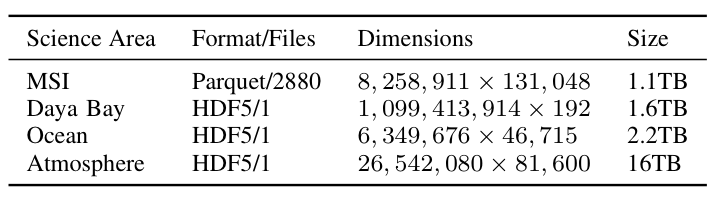
Table 1: Descriptions of the data sets used in our experiments.
For each decomposition, we implemented the same algorithms for PCA, NMF, and CX in C+MPI and in Spark. Our data sets are all “tall-and-skinny” highly rectangular matrices. We used H5Spark, a Spark interface to the HDF5 library developed at NERSC, to load the HDF5 files. The end-to-end (including IO) compute times for the Spark codes and the MPI codes are summarized in Table 2 for different levels of concurrency.
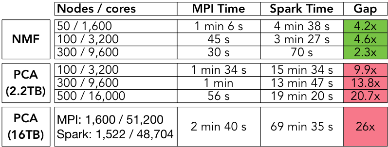
Table 2: summary of Spark and MPI run-times.
The MPI codes range from 2 to 26 times faster than the Spark codes for PCA and NMF. The performance gap is lowest for the NMF algorithm at the highest level of concurrency, and highest for the PCA algorithm at the highest level of concurrency. Briefly, this difference is due to the fact that our NMF algorithm makes one pass over the dataset, so IO is the dominant cost, and this cost decreases as concurrency increases. On the other hand, the PCA algorithm is an iterative algorithm (Lanczos), which makes multiple passes over the dataset, so the dominant cost is due to synchronization and scheduling; these costs increase with the level of concurrency.
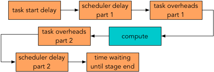
Figure 1: Spark overheads.
Figure 1 summarizes some sources of Spark overhead during each task. Here, “task start delay” measures the time from the start of the stage to the time the task reaches the executor; “scheduler delay” is the time between a task being received and being deserialized plus the time between result serialization and the driver receiving the task’s completion message; “task overhead time” measures the time spent waiting on fetches, executor deserialization, shuffle writing, and serializing results; and “time waiting until stage end” is the time spent waiting for all other tasks in the stage to end.
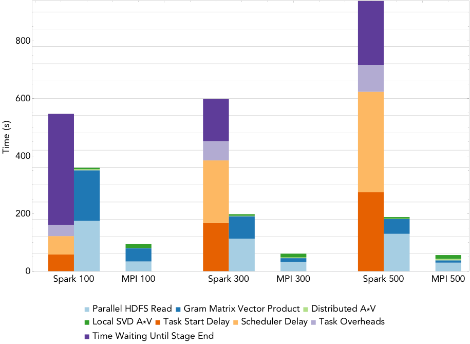
Figure 2: Run times for rank 20 PCA decomposition of the 2.2TB ocean temperature data set on varying number of nodes.
To compute the PCA, we use an iterative algorithm that computes a series of distributed matrix-vector products until convergence to the decomposition is achieved. As the rank of the desired decomposition rises, the number of required matrix-vector products increases. Figure 2 shows the run times for the MPI and Spark codes when computing a rank 20 PCA of the 2.2TB ocean temperature data set on NERSC’s Cori supercomputer, as the level of parallelism increases from 100 nodes (3,200 cores) to 500 nodes (16,000 cores). The overheads are reported as the sum over all stages of the mean overheads for the tasks in each stage. The remaining buckets are computational stages common to both the Spark and MPI implementations. We can see that that the dominant costs of computing the PCA here is the cost of synchronizing and scheduling the distributed matrix-vector products, and these costs increase with the level of concurrency. Comparing just the compute phases, Spark is less than 4 times slower than MPI at all levels of concurrency, with this gap decreasing as concurrency increases.
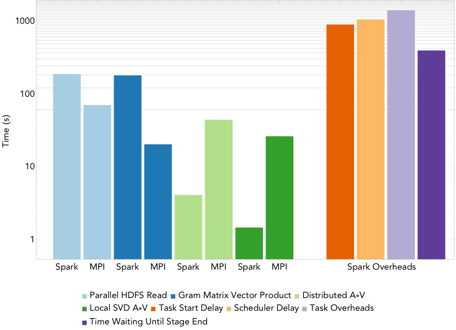
Figure 3: Run times for computing a rank 20 decomposition of the 16TB atmospheric humidity data set on 1522/1600 nodes.
Figure 3 shows the run times for the MPI and Spark codes for PCA at a finer level of granularity for the largest PCA run, computing a rank 20 decomposition of a 16TB atmospheric humidity matrix on 1600 of the 1630 nodes of the Cori supercomputer at NERSC. MPI scaled successfully to all 51200 cores, and Spark managed to launch 1522 of the requested executors, so scaled to 48704 cores. The running time for the Spark implementation is 1.2 hours while that for the MPI implementation is 2.7 minutes. Thus, for this PCA algorithm, Spark’s performance is not comparable to MPI— we note that the algorithm we implemented is the same as the most scalable PCA algorithm currently available in MLlib.
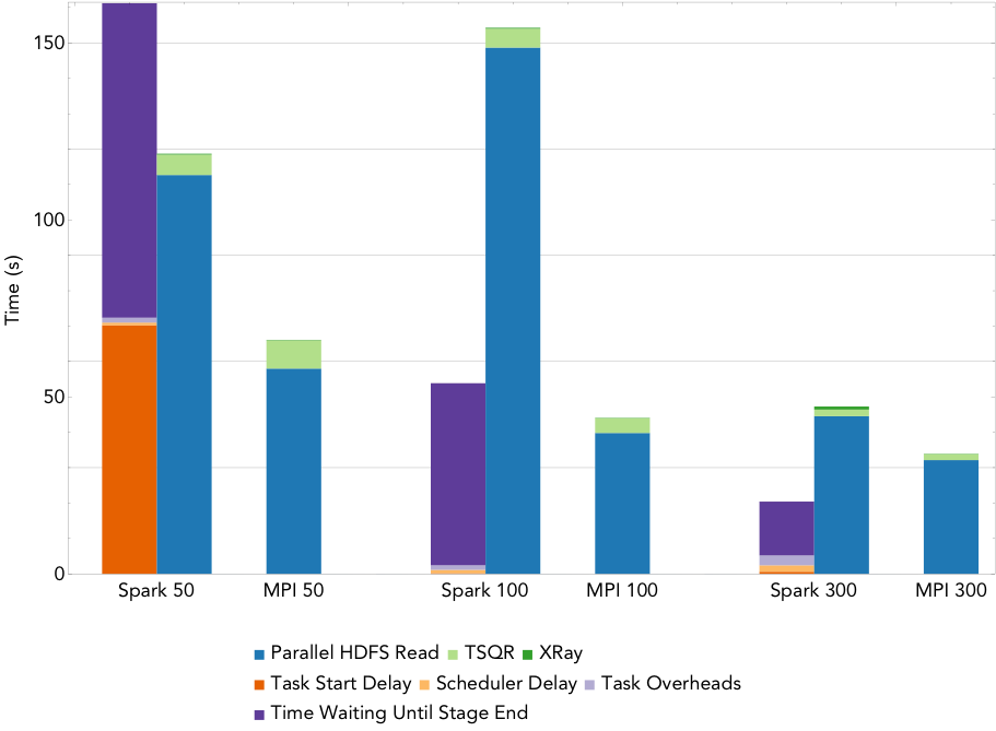
Figure 4: Run times for NMF decomposition of the 1.6TB Daya Bay data set on a varying number of nodes.
By way of comparison, the Spark NMF implementation scales much better. Figure 4 gives the run time breakdowns for NMF run on 50 nodes, 100 nodes, and 300 nodes of Cori (1,600, 3,2000, and 16,000 cores respectively). This implementation uses a slightly modified version of the tall-skinny QR algorithm (TSQR) available in ml-matrix to reduce the dimensionality of the input matrix, and computes the NMF on this much smaller matrix locally on the driver. The TSQR is computed in one pass over the matrix, so the synchronization and scheduling overheads are minimized, and the dominant cost is the IO. The large task start delay in the 50 node case is due to the fact that the cluster is not large enough to hold the entire matrix in memory.
The performance of the CX decomposition falls somewhere in between that of the PCA and the NMF, because the algorithm involves only a few passes (5) over the matrix. Our investigation into the breakdown of the Spark overheads (and how they might be mitigated with more carefully designed algorithms) is on-going. We are also collaborating with climate scientists at LBL in the analysis of the three-dimensional climate trends extracted from the CFSR data.

This is a guest blog post originally published on the Databricks blog.
For the past few months, we have been busy working on the next major release of the big data open source software we love: Apache Spark 2.0. Since Spark 1.0 came out two years ago, we have heard praises and complaints. Spark 2.0 builds on what we have learned in the past two years, doubling down on what users love and improving on what users lament. While this blog summarizes the three major thrusts and themes—easier, faster, and smarter—that comprise Spark 2.0, the themes highlighted here deserve deep-dive discussions that we will follow up with in-depth blogs in the next few weeks.
Prior to the general release, a technical preview of Apache Spark 2.0 is available on Databricks. This preview package is built using the upstream branch-2.0. Using the preview package is as simple as selecting the “2.0 (branch preview)” version when launching a cluster.
Whereas the final Apache Spark 2.0 release is still a few weeks away, this technical preview is intended to provide early access to the features in Spark 2.0 based on the upstream codebase. This way, you can satisfy your curiosity to try the shiny new toy, while we get feedback and bug reports early before the final release.
Now, let’s take a look at the new developments.

One thing we are proud of in Spark is creating APIs that are simple, intuitive, and expressive. Spark 2.0 continues this tradition, with focus on two areas: (1) standard SQL support and (2) unifying DataFrame/Dataset API.
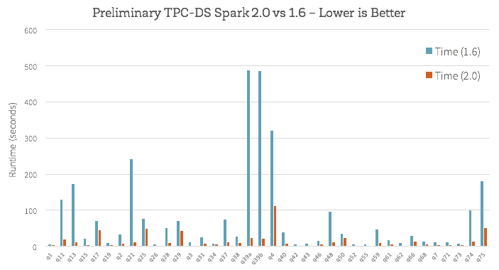
On the SQL side, we have significantly expanded the SQL capabilities of Spark, with the introduction of a new ANSI SQL parser and support for subqueries. Spark 2.0 can run all the 99 TPC-DS queries, which require many of the SQL:2003 features. Because SQL has been one of the primary interfaces Spark applications use, this extended SQL capabilities drastically reduce the porting effort of legacy applications over to Spark.
On the programming API side, we have streamlined the APIs:
map, filter, groupByKey) and the untyped methods (e.g. select, groupBy) are available on the Dataset class. Also, this new combined Dataset interface is the abstraction used for Structured Streaming. Since compile-time type-safety in Python and R is not a language feature, the concept of Dataset does not apply to these languages’ APIs. Instead, DataFrame remains the primary programing abstraction, which is analogous to the single-node data frame notion in these languages. Get a peek from a Dataset API notebook.According to our 2015 Spark Survey, 91% of users consider performance as the most important aspect of Spark. As a result, performance optimizations have always been a focus in our Spark development. Before we started planning for Spark 2.0, we asked ourselves a question: Spark is already pretty fast, but can we push the boundary and make Spark 10X faster?
This question led us to fundamentally rethink the way we build Spark’s physical execution layer. When you look into a modern data engine (e.g. Spark or other MPP databases), majority of the CPU cycles are spent in useless work, such as making virtual function calls or reading/writing intermediate data to CPU cache or memory. Optimizing performance by reducing the amount of CPU cycles wasted in these useless work has been a long time focus of modern compilers.
Spark 2.0 ships with the second generation Tungsten engine. This engine builds upon ideas from modern compilers and MPP databases and applies them to data processing. The main idea is to emit optimized bytecode at runtime that collapses the entire query into a single function, eliminating virtual function calls and leveraging CPU registers for intermediate data. We call this technique “whole-stage code generation.”
To give you a teaser, we have measured the amount of time (in nanoseconds) it would take to process a row on one core for some of the operators in Spark 1.6 vs. Spark 2.0, and the table below is a comparison that demonstrates the power of the new Tungsten engine. Spark 1.6 includes expression code generation technique that is also in use in some state-of-the-art commercial databases today. As you can see, many of the core operators are becoming an order of magnitude faster with whole-stage code generation.
You can see the power of whole-stage code generation in action in this notebook, in which we perform aggregations and joins on 1 billion records on a single machine.
| primitive | Spark 1.6 | Spark 2.0 |
|---|---|---|
| filter | 15ns | 1.1ns |
| sum w/o group | 14ns | 0.9ns |
| sum w/ group | 79ns | 10.7ns |
| hash join | 115ns | 4.0ns |
| sort (8-bit entropy) | 620ns | 5.3ns |
| sort (64-bit entropy) | 620ns | 40ns |
| sort-merge join | 750ns | 700ns |
How does this new engine work on end-to-end queries? We did some preliminary analysis using TPC-DS queries to compare Spark 1.6 and Spark 2.0:
Beyond whole-stage code generation to improve performance, a lot of work has also gone into improving the Catalyst optimizer for general query optimizations such as nullability propagation, as well as a new vectorized Parquet decoder that has improved Parquet scan throughput by 3X.
Spark Streaming has long led the big data space as one of the first attempts at unifying batch and streaming computation. As a first streaming API called DStream and introduced in Spark 0.7, it offered developers with several powerful properties: exactly-once semantics, fault-tolerance at scale, and high throughput.
However, after working with hundreds of real-world deployments of Spark Streaming, we found that applications that need to make decisions in real-time often require more than just a streaming engine. They require deep integration of the batch stack and the streaming stack, integration with external storage systems, as well as the ability to cope with changes in business logic. As a result, enterprises want more than just a streaming engine; instead they need a full stack that enables them to develop end-to-end “continuous applications.”
One school of thought is to treat everything like a stream; that is, adopt a single programming model integrating both batch and streaming data.
A number of problems exist with this single model. First, operating on data as it arrives in can be very difficult and restrictive. Second, varying data distribution, changing business logic, and delayed data—all add unique challenges. And third, most existing systems, such as MySQL or Amazon S3, do not behave like a stream and many algorithms (including most off-the-shelf machine learning) do not work in a streaming setting.
Spark 2.0’s Structured Streaming APIs is a novel way to approach streaming. It stems from the realization that the simplest way to compute answers on streams of data is to not having to reason about the fact that it is a stream. This realization came from our experience with programmers who already know how to program static data sets (aka batch) using Spark’s powerful DataFrame/Dataset API. The vision of Structured Streaming is to utilize the Catalyst optimizer to discover when it is possible to transparently turn a static program into an incremental execution that works on dynamic, infinite data (aka a stream). When viewed through this structured lens of data—as discrete table or an infinite table—you simplify streaming.
As the first step towards realizing this vision, Spark 2.0 ships with an initial version of the Structured Streaming API, a (surprisingly small!) extension to the DataFrame/Dataset API. This unification should make adoption easy for existing Spark users, allowing them to leverage their knowledge of Spark batch API to answer new questions in real-time. Key features here will include support for event-time based processing, out-of-order/delayed data, sessionization and tight integration with non-streaming data sources and sinks.
Streaming is clearly a pretty broad topic, so stay tuned to this blog for more details on Structured Streaming in Spark 2.0, including details on what is possible in this release and what is on the roadmap for the near future.
Spark users initially came to Spark for its ease-of-use and performance. Spark 2.0 doubles down on these while extending it to support an even wider range of workloads. We hope you will enjoy the work we have put it in, and look forward to your feedback.
Of course, until the upstream Apache Spark 2.0 release is finalized, we do not recommend fully migrating any production workload onto this preview package. This technical preview version is now available on Databricks. You can sign up for an account here.
If you missed our webinar for Spark 2.0: Easier, Faster, and Smarter, you can register and watch the recordings and download slides and attached notebooks.
You can also import the following notebooks and try on Databricks Community Edition with Spark 2.0 Technical Preview.
I am very pleased to announce that Julian Shun has been awarded the ACM’s doctoral dissertation award for his 2015 CMU doctoral thesis “Shared-Memory Parallelism Can Be Simple, Fast, and Scalable” which also won that year’s CMU SCS distinguished dissertation award.
Julian currently works with me as a postdoc both in the Department of Statistics and in the AMP Lab in the EECS Department and is supported by a Miller Fellowship. His research focuses on fundamental theoretical and practical questions at the interface between computer science and statistics for large-scale data analysis. He is particularly interested in all aspects of parallel computing, especially parallel graph processing frameworks, algorithms, data structures and tools for deterministic parallel programming; and he has developed Ligra, a lightweight graph processing framework for shared memory.
More details can be found in the official ACM announcement.
Join me in congratulating Julian!

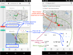
So this is really weird, but I have found what seems to be unexpected continuous location tracking that is causing noticeable battery drain on Android 6.0. Right now, it’s looking like a change in an automatically updated component, so it is probably due to a closed source service or app. So this is in the style of the work from Vern Paxson’s group on characterizing the observed behavior of third party software.
Has anybody else running Android 6.0 noticed a particularly large increase in power drain, with the GPS icon displayed continuously? I will be running additional tests in the coming days, but wanted to report the unusual behavior and see if other researchers have noticed it as well, or want to investigate it while it lasts.
I’ve been doing power profiling of power drain under various regimes as part of understanding the power/accuracy tradeoffs for my travel pattern tracking project. So I basically install apps with different data collection regimes on multiple test phones of the same make, model and OS version, and carry all of them around for comparison.
From last Thu/Fri/Sat, it looks like the power drain behavior on android has changed dramatically. In particular, it looks like some system component has GPS location turned on continuously, and is draining the battery quite dramatically. See details below.
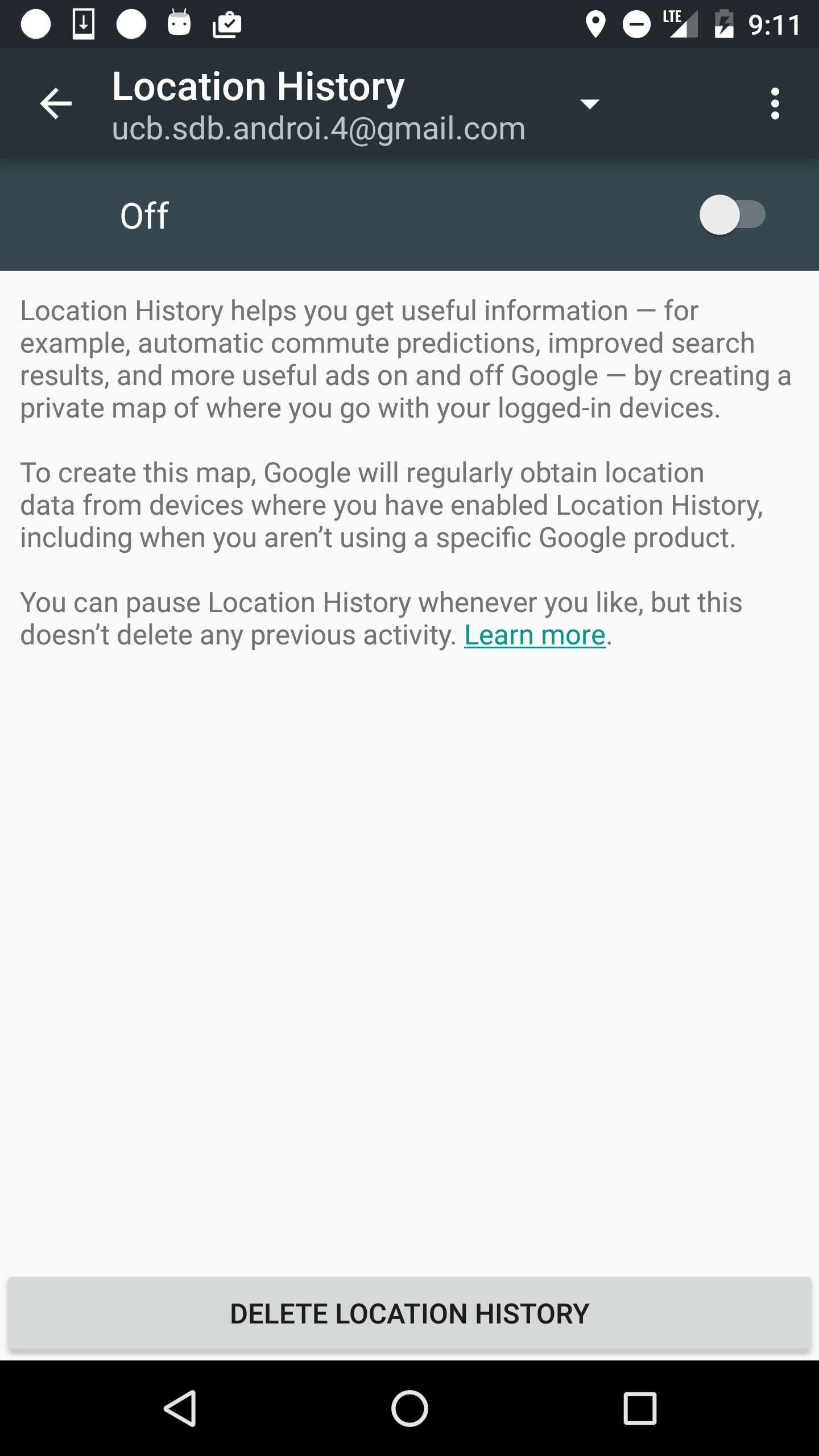
This is a Nexus 6 running a stock android kernel (v 6.0.1, patch level: March 1, 2016), with no non-OEM apps installed other than mine, and with google maps location history turned off, so this must be due to unexpected background access by either the OS or some stock google app. And since I didn’t update the OS, my guess is that it is a closed source component such as google play services or google maps that is automatically updated/patched.
| Phone 1 | Phone 2 | Phone 3 | Phone 4 | |
| Sat | tracking off | tracking off | tracking off | tracking off |
| Tue | high, 1 sec | med, 1 sec | high, 15-30 sec | med, 15-30 sec |
| Thu | high, 1 sec | med, 1 sec | high, 30 sec | tracking off |
| Fri + Sat | high, 1 sec | med, 1 sec | high, 30 sec | tracking off |
| Next Tue | high, 1 sec | med, 1 sec | high, 30 sec | tracking off |

It is clear that on Tuesday, phones 2 and 3 are fairly close to each other, and both are very different from phone 1. This is consistent with intuition and results before Thursday as well.
On Thursday, the difference between phone 1 and phone 2 is much less pronounced, and the difference between phone 2 and phone 3 is also much larger. On Friday and this Tuesday, there is essentially no difference between high and medium accuracy at the fast sampling rate (phone 1 and phone 2), and no difference between slow sampling and no tracking (phone 3 and phone 4).
Of course, this could be a bug in my code, but:
This is complicated because we are trying to treat the phone like a natural phenomenon that we cannot control but can try to understand through observation. I’d love to hear from other members of the community so that we can figure out whether google is really continuously tracking us without letting us know, and killing our battery while doing so.

The Strata+Hadoop World big data industry conference was held in San Jose this week and as usual, AMPLab and Berkeley were well-represented among the presentations, while uniquely among university projects, AMPLab alumni and AMPLab-developed software were prominent throughout the conference. I got the opportunity to give an update on the BDAS stack in a short Keynote talk to the (I’m guessing) 2500 or so people who got up early enough to attend the morning session on Thursday. Scheduled between a talk on brain surgery and a stand up improv routine by Paula Poundstone (of NPR’s “Wait Wait, Don’t Tell Me“) and after a nice introduction from long-time AMPLab friend and supporter Ben Lorica, I gave a quick over view of the AMPLab and BDAS, and then focused on four of our ongoing projects: Succinct, Velox, KeystoneML, and AMPCrowd/SampleClean.
O’Reilly, the sponsor of Strata, has put videos of the keynotes on line (free, but log-in required). The keynote I gave can be viewed here. Thanks to everyone who provided slides for and advice on the presentation.

Hoping to start a new tradition, I’m giving a Last Lecture on Friday May 6, 2016 at 4PM, which is shortly before I retire. (The premise of these is that if this were the last public lecture you would give, what would you say.) My title is “How to Be a Bad Professor” (abstract), and it is followed by a reception.
There will also be a one-day symposium on Saturday May 7 (agenda) with talks by colleagues and former students on the future of topics associated with my 40 years at UC Berkeley, such as the microprocessors, storage, cloud computing, data science, and machine learning.
Both events will be held at the International House at UC Berkeley.
Please sign up to the event of interest, and feel free to invite other interested parties.
Dave
P.S. Those who sign up before April 7 for the symposium will get a commemorative book with perspectives by Stanford President John Hennessy, National Medal of Science Winner Richard Tapia, former UCSC Chancellor Karl Pister, and other luminaries.

At the AMPLab, we are constantly looking for ways to improve the performance and user experience of large scale advanced analytics. We frequently make the fruits of our research available as open source software. Last week, we released version 0.3 of KeystoneML, a project we’ve blogged about in the past. KeystoneML is designed to simplify the construction of large scale end-to-end machine learning pipelines. For this development cycle, we focused our efforts on pipeline optimization including new features to automatically materialize intermediate reused state and cost-based selection of logical pipeline operators. In this post, we’ll recap how users can describe machine learning applications using high-level operators with KeystoneML. Then, we’ll discuss how the new features in the latest release accelerate the training of these applications.
In KeystoneML, users describe their machine learning applications as the composition of high level, modular components, which can be chained together to form complex pipeline DAGs. These components can range from general purpose statistical transformations and machine learning algorithms, to domain-specific featurization techniques (e.g., from image processing), to user-defined operations. Here’s a simple example of a text classification application specified using KeystoneML:
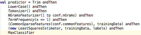
In this code snippet, a pipeline for text classification does initial pre-processing of the text using simple nodes (for example, Trim, Lowercase), converts the processed text to a vector space representation, and then fit a least squares classifier on it. Note, however, that this is an abstract definition of the classification process: the pipeline is defined independently of the actual implementation of any of its components, and the user does not need to specify how they want this application trained. This is where the KeystoneML optimizer and the new features in v0.3 come in.
Physical Operator Selection: Given the above abstract pipeline definition, one important consideration is physical operator selection. In the case of the LeastSquaresEstimator, for example, there are multiple ways to solve a linear system, and which method is best will depend on characteristics of the data (number of examples, number of features, sparsity) and the hardware (size of your cluster, how many cores, how fast is the network). In KeystoneML, a cost-based optimizer selects the appropriate physical operator to use when fitting the model based on these statistics. We refer to these kinds of optimizations as node-level optimizations.
Automatic Caching: Another class of optimizations that we have developed is whole-pipeline optimization. Given the above pipeline definition, we might use an iterative algorithm to solve the least squares problem. In this case, the algorithm will read its inputs many times before emitting a model. In this setting, it may make a lot of sense to cache the input just before the solve. But, if the input features are too big to cache fully, perhaps an earlier stage in the pipeline is an appropriate place to cache. These kinds of decisions can be tough for users to make, particularly in the face of changing workloads. Fortunately, the optimizer in KeystoneML v0.3 contains logic to automatically select which intermediate state(s) to cache.
New Operators: We’ve included a number of new Operators in this release. These include a Scala-native GMM implementation which is faster than the existing C-version for small numbers of Gaussians, a node for Image Cropping, the hashing trick for text featurization, summary information for binary classifiers, and a variety of implementations of PCA. In particular, we’ve included both local and distributed PCA implementations, as well as a distributed approximate PCA algorithm which can be significantly faster than the exact algorithm when the number of principal components requested is small relative to the number of features in the matrix.
In this post we’ve highlighted some of the new features in KeystoneML v0.3. For more information check the release notes. Also, KeystoneML v0.3 will be a focus of Mike Franklin’s keynote talk at the Strata conference on Thursday morning later this week. We are already hard at work on KeystoneML v0.4, including work on large scale kernel methods, advanced hyperparameter tuning support, and sophisticated job placement and cluster sizing algorithms. We look forward to your feedback and feature requests on Github.